Saturday, November 29, 2014

Dimension Reduction using spectral decomposition (1) - LDA


Introduction

Most of texts including textbooks and web articles describe FLD(Fisher Linear Discriminant) as LDA instead of classical LDA. However if you survey academical papers released 10 years ago, you will find more simpler LDA than FLD.

The issues that LDA concerns are totally different from PCA's. The concept of "group or class" is added into LDA. PCA deals with individual samples. LDA focuses on classifications of sample groups.

PCA can be used as a recognition/classification approach by itself. But actually PCA is used as preprocessing of dimention reduction for more complex methods for classification or recognition. And some strategy used in PCA process is already melt inside LDA.

My reference on web is :
  1. https://onlinecourses.science.psu.edu/stat557/node/37
  2. http://en.wikipedia.org/wiki/Linear_discriminant_analysis
Before discussion on LDA, I will explain Mahalanobis Distance and Multivariate Normal Distribution. And then QDA, complicated version of LDA. Finally LDA. All of things in this articles are based on simillar process using covariance matrix.

Unfortunately this classical LDA needs 2 strict assumptions, identical covaraince matrix and multivariate normal distribution. They make hard to apply LDA on real world problems. But its strategy is simple. and through traveling to LDA here, we can understand relationships between a lot of contents look simillar but never explained in one shot.


Euclidean Distance and Mahalanobis Distance

There are so many types of distance metric between two vectors or features. Euclidean Distance is the simplest.
\begin{equation} D_{Euclidean}(\mathbf{x})=\sqrt{(\mathbf{x}-\mathbf{y})^{T}(\mathbf{x}-\mathbf{y})} \end{equation}

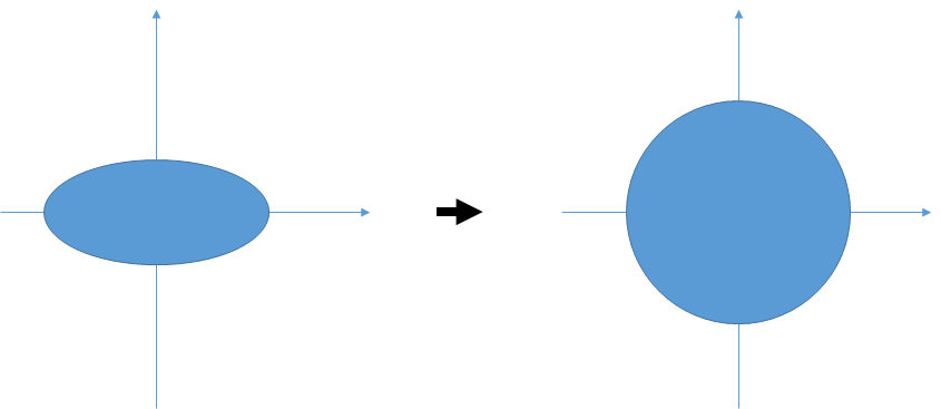
As describe in the figure above, if we select euclidean distance, we don't care about the distribution of sample group and its covariances.

 
In the calculation of Mahalanobis Distance, normalization transform on bases is added just before Euclidean Distance calculation.
\begin{equation} D_{Mahalanobis}(\mathbf{x})=\sqrt[]{(\mathbf{x}-\mathbf{y})^{T}\mathbf{\Sigma}^{-1}(\mathbf{x}-\mathbf{y})} \end{equation}


Let's deep-dive into the $\Sigma^-1$.
We already look over covariance matrix $\Sigma$ in the previous article of PCA.

\begin{eqnarray*} \Sigma & = & \left[\begin{array}{ccc} \sigma_{11}^{2} & \cdots & \sigma_{1D}^{2}\\ \vdots & \ddots & \vdots\\ \sigma_{D1}^{2} & \cdots & \sigma_{DD}^{2} \end{array}\right]\\ & \Downarrow & diagonalization\\ & = & Q\varLambda Q^{T}\\ & = & \left[\begin{array}{cccc} \mathbf{e}_{1} & \mathbf{e}_{2} & \cdots & \mathbf{e}_{D}\end{array}\right]\left[\begin{array}{ccc} \lambda_{1} & \cdots & 0\\ \vdots & \ddots & \vdots\\ 0 & \cdots & \lambda_{D} \end{array}\right]\left[\begin{array}{c} \mathbf{e}_{1}^{T}\\ \mathbf{e}_{2}^{T}\\ \vdots\\ \mathbf{e}_{D}^{T} \end{array}\right] \end{eqnarray*}

$\lambda$s can be replaced with "NEW" variances, $\sigma^2$s.

\begin{eqnarray*} \Sigma & = & Q\varLambda Q^{T}\\ & = & \left[\begin{array}{cccc} \mathbf{e}_{1} & \mathbf{e}_{2} & \cdots & \mathbf{e}_{D}\end{array}\right]\left[\begin{array}{ccc} \sigma_{11}^{2} & \cdots & 0\\ \vdots & \ddots & \vdots\\ 0 & \cdots & \sigma{}_{DD}^{2} \end{array}\right]\left[\begin{array}{c} \mathbf{e}_{1}^{T}\\ \mathbf{e}_{2}^{T}\\ \vdots\\ \mathbf{e}_{D}^{T} \end{array}\right] \end{eqnarray*}
 
The matrix consisting of $\mathbf{e}^T_d$s means transformation to new bases ${\mathbf{e}_d}$.


\begin{eqnarray*} \Sigma^{-1} & = & Q\varLambda^{-1}Q^{T}\\ & = & \left[\begin{array}{cccc} \mathbf{e}_{1} & \mathbf{e}_{2} & \cdots & \mathbf{e}_{D}\end{array}\right]\left[\begin{array}{ccc} \frac{1}{\sigma{}_{11}^{2}} & \cdots & 0\\ \vdots & \ddots & \vdots\\ 0 & \cdots & \frac{1}{\sigma{}_{DD}^{2}} \end{array}\right]\left[\begin{array}{c} \mathbf{e}_{1}^{T}\\ \mathbf{e}_{2}^{T}\\ \vdots\\ \mathbf{e}_{D}^{T} \end{array}\right]\\ & = & \left(\left[\begin{array}{cccc} \mathbf{e}_{1} & \mathbf{e}_{2} & \cdots & \mathbf{e}_{D}\end{array}\right]\left[\begin{array}{ccc} \frac{1}{\sigma{}_{11}} & \cdots & 0\\ \vdots & \ddots & \vdots\\ 0 & \cdots & \frac{1}{\sigma{}_{DD}} \end{array}\right]\right)\left(\left[\begin{array}{ccc} \frac{1}{\sigma{}_{11}} & \cdots & 0\\ \vdots & \ddots & \vdots\\ 0 & \cdots & \frac{1}{\sigma{}_{DD}} \end{array}\right]\left[\begin{array}{c} \mathbf{e}_{1}^{T}\\ \mathbf{e}_{2}^{T}\\ \vdots\\ \mathbf{e}_{D}^{T} \end{array}\right]\right) \end{eqnarray*}

$\frac{1}{\sigma}$ means unit-varaince normalization.


Multivariate Normal Distribution

Multivariate Normal Distribution(MND) is :

\begin{equation} \mathcal{N}_{D}(\mu,\Sigma)=\frac{1}{\sqrt{2\pi^{D}\left|\Sigma\right|}}\exp\left(-\frac{1}{2}(\mathbf{x}-\mu)^{T}\mathbf{\Sigma}^{-1}(\mathbf{x}-\mu)\right) \end{equation}

where $D=\dim\left(\mathbf{x}\right)$.

We can see a term of squared Mahalanobis Distance. $(\mathbf{x}-\mu)^T\Sigma^{-1}(\mathbf{x}-\mu)$ means the squared Mahalanobis Distance from $\mu$. Determinant of $\Sigma$ is a product of variances $\prod_{d}\sigma_d^2$.


QDA (Quadratic Discriminant Analysis)

QDA is more general form of LDA. For QDA We need a important assumption that all classes have a normal distribution (MND).


If we want to discriminate class k and h, we have the following discriminant system.

\begin{equation} \frac{g_{k}(\mathbf{x})}{g_{h}(\mathbf{x})}>T_{k\text{ against }h} \end{equation} \begin{eqnarray*} g_{k}(\mathbf{x}) & = & p(\mathbf{x}|C_{k})p(C_{k})\\ & = & \frac{1}{\sqrt{2\pi^{D}\left|\Sigma_{k}\right|}}\exp\left(-\frac{1}{2}(\mathbf{x}-\mu_{k})^{T}\mathbf{\Sigma}_{k}^{-1}(\mathbf{x}-\mu_{k})\right)p(C_{k}) \end{eqnarray*} \begin{eqnarray*} \frac{g_{k}(\mathbf{x})}{g_{h}(\mathbf{x})} & = & \frac{\frac{1}{\sqrt{2\pi^{D}\left|\Sigma_{k}\right|}}\exp\left(-\frac{1}{2}(\mathbf{x}-\mu_{k})^{T}\mathbf{\Sigma}_{k}^{-1}(\mathbf{x}-\mu_{k})\right)p(C_{k})}{\frac{1}{\sqrt{2\pi^{D}\left|\Sigma_{h}\right|}}\exp\left(-\frac{1}{2}(\mathbf{x}-\mu_{h})^{T}\mathbf{\Sigma}_{h}^{-1}(\mathbf{x}-\mu_{h})\right)p(C_{h})}\\ & = & \frac{\left|\Sigma_{k}\right|^{-\frac{1}{2}}\exp\left(-\frac{1}{2}(\mathbf{x}-\mu_{k})^{T}\mathbf{\Sigma}_{k}^{-1}(\mathbf{x}-\mu_{k})\right)p(C_{k})}{\left|\Sigma_{h}\right|^{-\frac{1}{2}}\exp\left(-\frac{1}{2}(\mathbf{x}-\mu_{h})^{T}\mathbf{\Sigma}_{h}^{-1}(\mathbf{x}-\mu_{h})\right)p(C_{h})} \end{eqnarray*}

It is based on simple Bayesian Decision. Let's refine the formula by using log-scale and the general notation, $\pi_{k}=p(C_{k})$

\begin{eqnarray*} \ln\left(\frac{g_{k}(\mathbf{x})}{g_{h}(\mathbf{x})}\right) & = & -\frac{1}{2}\ln\left|\Sigma_{k}\right|+\left(-\frac{1}{2}(\mathbf{x}-\mu_{k})^{T}\mathbf{\Sigma}_{k}^{-1}(\mathbf{x}-\mu_{k})\right)+\ln\pi_{k}+\frac{1}{2}\ln\left|\Sigma_{h}\right|-\left(-\frac{1}{2}(\mathbf{x}-\mu_{h})^{T}\mathbf{\Sigma}_{h}^{-1}(\mathbf{x}-\mu_{h})\right)-\ln\pi_{h} \end{eqnarray*}

The discriminant function has a quadratic form of vectors. This shows why its name is "Q"DA.


LDA (Linear Discriminant Analysis)

LDA need one more assumption. $\Sigma$s are same.

It looks unrealistics. But here go ahead.

\begin{eqnarray*} \ln\left(\frac{g_{k}(\mathbf{x})}{g_{h}(\mathbf{x})}\right) & = & -\frac{1}{2}\ln\left|\Sigma\right|+\left(-\frac{1}{2}(\mathbf{x}-\mu_{k})^{T}\mathbf{\Sigma}^{-1}(\mathbf{x}-\mu_{k})\right)+\ln\pi_{k}+\frac{1}{2}\ln\left|\Sigma\right|-\left(-\frac{1}{2}(\mathbf{x}-\mu_{h})^{T}\mathbf{\Sigma}^{-1}(\mathbf{x}-\mu_{h})\right)-\ln\pi_{h}\\ & = & \left(-\frac{1}{2}(\mathbf{x}-\mu_{k})^{T}\mathbf{\Sigma}^{-1}(\mathbf{x}-\mu_{k})\right)+\ln\pi_{k}-\left(-\frac{1}{2}(\mathbf{x}-\mu_{h})^{T}\mathbf{\Sigma}^{-1}(\mathbf{x}-\mu_{h})\right)-\ln\pi_{h}\\ & = & -\frac{1}{2}\left(\mathbf{x}^{T}\mathbf{\Sigma}^{-1}\mathbf{x}-2\mu_{k}^{T}\mathbf{\Sigma}^{-1}\mathbf{x}+\mu_{k}^{T}\mathbf{\Sigma}^{-1}\mu_{k}\right)+\frac{1}{2}\left(\mathbf{x}^{T}\mathbf{\Sigma}^{-1}\mathbf{x}-2\mu_{h}^{T}\mathbf{\Sigma}^{-1}\mathbf{x}+\mu_{h}^{T}\mathbf{\Sigma}^{-1}\mu_{h}\right)+\ln\pi_{k}-\ln\pi_{h}\\ & = & -\frac{1}{2}\left(-2\mu_{k}^{T}\mathbf{\Sigma}^{-1}\mathbf{x}+\mu_{k}^{T}\mathbf{\Sigma}^{-1}\mu_{k}\right)+\frac{1}{2}\left(-2\mu_{h}^{T}\mathbf{\Sigma}^{-1}\mathbf{x}+\mu_{h}^{T}\mathbf{\Sigma}^{-1}\mu_{h}\right)+\ln\pi_{k}-\ln\pi_{h}\\ & = & (\mu_{k}-\mu_{h})^{T}\mathbf{\Sigma}^{-1}\mathbf{x}-\frac{1}{2}(\mu_{k}+\mu_{h})^{T}\mathbf{\Sigma}^{-1}(\mu_{h}-\mu_{k})+\ln\pi_{k}-\ln\pi_{h} \end{eqnarray*}

As you see, the discriminant boundary changes from a curve to a straight line (Linear)


Conclusion

Covariance matrix is everywhere. The contents described here are so feasible that most of researchers and developers do not need to check again. But someone who doesn't have concrete mathematical or statistical funcdamentals cannot catch these common pieces and can be confused easily.

Syntax-Highlighter on blogspot

  • Select "Template" in Setting
  • "Edit HTML"

  • Add the following code in <head> </head>


<link href="http://alexgorbatchev.com/pub/sh/current/styles/shCore.css" rel="stylesheet" type="text/css"></link>
<link href="http://alexgorbatchev.com/pub/sh/current/styles/shThemeEmacs.css" rel="stylesheet" type="text/css"></link>
<script src="http://alexgorbatchev.com/pub/sh/current/scripts/shCore.js" type="text/javascript">
 
<script src='http://alexgorbatchev.com/pub/sh/current/scripts/shBrushAS3.js' type='text/javascript'/>
<script src='http://alexgorbatchev.com/pub/sh/current/scripts/shBrushBash.js' type='text/javascript'/>
<script src='http://alexgorbatchev.com/pub/sh/current/scripts/shBrushColdFusion.js' type='text/javascript'/>
<script src='http://alexgorbatchev.com/pub/sh/current/scripts/shBrushCSharp.js' type='text/javascript'/>
<script src='http://alexgorbatchev.com/pub/sh/current/scripts/shBrushCpp.js' type='text/javascript'/>
<script src='http://alexgorbatchev.com/pub/sh/current/scripts/shBrushCss.js' type='text/javascript'/>
<script src='http://alexgorbatchev.com/pub/sh/current/scripts/shBrushDelphi.js' type='text/javascript'/>
<script src='http://alexgorbatchev.com/pub/sh/current/scripts/shBrushDiff.js' type='text/javascript'/>
<script src='http://alexgorbatchev.com/pub/sh/current/scripts/shBrushErlang.js' type='text/javascript'/>
<script src='http://alexgorbatchev.com/pub/sh/current/scripts/shBrushGroovy.js' type='text/javascript'/>
<script src='http://alexgorbatchev.com/pub/sh/current/scripts/shBrushJScript.js' type='text/javascript'/>
<script src='http://alexgorbatchev.com/pub/sh/current/scripts/shBrushJava.js' type='text/javascript'/>
<script src='http://alexgorbatchev.com/pub/sh/current/scripts/shBrushJavaFX.js' type='text/javascript'/>
<script src='http://alexgorbatchev.com/pub/sh/current/scripts/shBrushPerl.js' type='text/javascript'/>
<script src='http://alexgorbatchev.com/pub/sh/current/scripts/shBrushPhp.js' type='text/javascript'/>
<script src='http://alexgorbatchev.com/pub/sh/current/scripts/shBrushPlain.js' type='text/javascript'/>
<script src='http://alexgorbatchev.com/pub/sh/current/scripts/shBrushPowerShell.js' type='text/javascript'/>
<script src='http://alexgorbatchev.com/pub/sh/current/scripts/shBrushPython.js' type='text/javascript'/>
<script src='http://alexgorbatchev.com/pub/sh/current/scripts/shBrushRuby.js' type='text/javascript'/>
<script src='http://alexgorbatchev.com/pub/sh/current/scripts/shBrushScala.js' type='text/javascript'/>
<script src='http://alexgorbatchev.com/pub/sh/current/scripts/shBrushSql.js' type='text/javascript'/>
<script src='http://alexgorbatchev.com/pub/sh/current/scripts/shBrushVb.js' type='text/javascript'/>
<script src='http://alexgorbatchev.com/pub/sh/current/scripts/shBrushXml.js' type='text/javascript'/>
  
<script language='javascript' type='text/javascript'>
 SyntaxHighlighter.config.bloggerMode = true;
 SyntaxHighlighter.all();
</script>
<!-- Syntax Highlighter Additions END -->
  •  Add the following javascript code at the end of every post in HTML mode
<pre class="brush:c;"><code>&lt;script type="text/javascript"&gt;
 SyntaxHighlighter.highlight();
&lt;/script&gt;</code>
</pre>

<script type="text/javascript">
 SyntaxHighlighter.highlight();
</script>

Dimension Reduction using spectral decomposition (0) - PCA


Introduction

I survey most of dimensional reduction methods by using spectral decomposition such as PCA(Principal Component Analysis), LDA(Linear Discriminant Analysis), FLD(Fischer Linear Discriminant), MDA(Multivariate Discriminant Analysis), CCA(Cannonical Correlation Analysis). The following description is in chronological order. Whenever we move to the next methodology, the conditions of problems are more complicated. There are so many articles about these methodology. But I could not found any report that focus on the relationship between methods. I need to know why our predecessors developed these:  from PCA to CCA or other more complicated method. My final goal is setup a unified  table of all methods using same mathematical notation for easier understanding.


Line Fitting on Sample Points

Before we start to discuss PCA, let's review typical line fitting problem ussing sum of squared errors.
All of basic machine learning methods are based on minimzing sum of squared errors.


Let's see a regression line $\mathbf{\mathbf{x}_{0}+}a\mathbf{e}$ (where $\left\Vert \mathbf{e}\right\Vert =1$ ) on the sample $\mathbf{x}_{n}$.

Objective function $f$ to minimize is : \begin{equation} f(\mathbf{x}_{0},\mathbf{e},a_{0},...a_{N})=\sum_{n}^{N}\left\Vert \mathbf{x}_{n}-(\mathbf{x}_{0}+a_{n}\mathbf{e})\right\Vert ^{2} \end{equation} where $\mathbf{x}_{0}+a_{n}\mathbf{e}$ is the closed point to $\mathbf{x}_{n}$ on the regression line.

This sum of squared errors (SSE) is just one among several candidates of cost functions. L1 norm or other norms can be the cost function. If a specific cost function of error is given, we must use it instead of SSE. The reason why most of standard methods use it is easy to handle the formula. SSE is differentiable, so we can analyze its parameters in closed form expressions. (c.f. In logistics regression we should do numerical analysis.)

I will check the relationship between the regression line and $\mu$, mean of $\mathbf{x}_{n}$.

At first, calculate the derivative of $a_{n}$in terms of $\mathbf{x}_{0},\mathbf{x}_{n},\mathbf{e}$. \begin{equation} f(\mathbf{x}_{0},\mathbf{e},a_{0},...a_{N})=\sum_{n}^{N}\left\Vert a_{n}\mathbf{e}+\mathbf{\mathbf{x}}_{0}-\mathbf{x}_{n}\right\Vert ^{2} \end{equation} \begin{eqnarray*} \frac{\partial f}{\partial a_{n}} & = & \frac{\partial\left(\sum_{n}^{N}\left\Vert a_{n}\mathbf{e}+\mathbf{\mathbf{x}}_{0}-\mathbf{x}_{n}\right\Vert ^{2}\right)}{\partial a_{n}}=\frac{\partial\left(\left\Vert a_{n}\mathbf{e}+\mathbf{\mathbf{x}}_{0}-\mathbf{x}_{n}\right\Vert ^{2}\right)}{\partial a_{n}}\\ & = & \frac{\partial\left(a_{n}^{2}\left\Vert \mathbf{e}\right\Vert ^{2}+2a_{n}\mathbf{e}^{T}(\mathbf{\mathbf{x}}_{0}-\mathbf{x}_{n})+\left\Vert \mathbf{\mathbf{x}}_{0}-\mathbf{x}_{n}\right\Vert ^{2}\right)}{\partial a_{n}}\\ & = & 2a_{n}+2\mathbf{e}^{T}(\mathbf{\mathbf{x}}_{0}-\mathbf{x}_{n}) \end{eqnarray*}

We can get $\underset{a_{n}}{\arg\min}(f)$ by ${\displaystyle \frac{\partial f}{\partial a_{n}}=0}$. \begin{equation} a_{n}=\mathbf{e}^{T}(\mathbf{\mathbf{x}}_{n}-\mathbf{x}_{0}) \end{equation}

This means that projection of $(\mathbf{\mathbf{x}}_{n}-\mathbf{x}_{0})$ on $\mathbf{e}$. Actually most of books skip this proof, since it is a basic linear algebra.

Now analyze $f$ with respect to $\mathbf{x}_{0}$.

In expanding $f$ I use $a_{n}$ instead of $\mathbf{e}^{T}(\mathbf{\mathbf{x}}_{n}-\mathbf{x}_{0})$ for a moment. It is just for easier calculation. \begin{eqnarray*} f(\mathbf{x}_{0},\mathbf{e}) & = & \sum_{n}^{N}\left\Vert \mathbf{x}_{0}-\mathbf{x}_{n}+a_{n}\mathbf{e}\right\Vert ^{2}\\ & = & \sum_{n}^{N}\left(\left\Vert \mathbf{x}_{0}-\mathbf{x}_{n}\right\Vert ^{2}+2(a_{n}\mathbf{e})^{T}(\mathbf{x}_{0}-\mathbf{x}_{n})+\left\Vert a_{n}\mathbf{e}\right\Vert ^{2}\right)\\ & = & \sum_{n}^{N}\left\Vert \mathbf{x}_{0}-\mathbf{x}_{n}\right\Vert ^{2}+2\sum_{n}^{N}a_{n}\overbrace{\left(\mathbf{e}{}^{T}(\mathbf{x}_{0}-\mathbf{x}_{n})\right)}^{=-a_{n}}+\sum_{n}^{N}a_{n}^{2}\overbrace{\left\Vert \mathbf{e}\right\Vert ^{2}}^{=1}\\ & = & \sum_{n}^{N}\left\Vert \mathbf{x}_{0}\right\Vert ^{2}-2\sum_{n}^{N}\mathbf{x}_{n}^{T}\mathbf{x}_{0}+\sum_{n}^{N}\left\Vert \mathbf{x}_{n}\right\Vert ^{2}-2\sum_{n}^{N}a_{n}(a_{n})+\sum_{n}^{N}a_{n}^{2}\\ & = & \sum_{n}^{N}\left\Vert \mathbf{x}_{0}\right\Vert ^{2}-2\sum_{n}^{N}\mathbf{x}_{n}^{T}\mathbf{x}_{0}+\sum_{n}^{N}\left\Vert \mathbf{x}_{n}\right\Vert ^{2}-\sum_{n}^{N}a_{n}^{2}\\ & = & \sum_{n}^{N}\left\Vert \mathbf{x}_{0}\right\Vert ^{2}-2\sum_{n}^{N}\mathbf{x}_{n}^{T}\mathbf{x}_{0}+\sum_{n}^{N}\left\Vert \mathbf{x}_{n}\right\Vert ^{2}-\sum_{n}^{N}(\mathbf{x}_{0}-\mathbf{x}_{n})^{T}\mathbf{e}\mathbf{e}^{T}(\mathbf{x}_{0}-\mathbf{x}_{n})\\ & = & N\left\Vert \mathbf{x}_{0}\right\Vert ^{2}-2\sum_{n}^{N}\mathbf{x}_{n}^{T}\mathbf{x}_{0}+\sum_{n}^{N}\left\Vert \mathbf{x}_{n}\right\Vert ^{2}-\sum_{n}^{N}\left(\mathbf{x}_{0}^{T}\mathbf{e}\mathbf{e}^{T}\mathbf{x}_{0}-2\mathbf{x}_{n}^{T}\mathbf{e}\mathbf{e}^{T}\mathbf{x}_{0}+\mathbf{x}_{n}^{T}\mathbf{e}\mathbf{e}^{T}\mathbf{x}_{n}\right)\\ & = & N\left\Vert \mathbf{x}_{0}\right\Vert ^{2}-\sum_{n}^{N}\mathbf{x}_{0}^{T}\mathbf{e}\mathbf{e}^{T}\mathbf{x}_{0}-2\sum_{n}^{N}\mathbf{x}_{n}^{T}\mathbf{x}_{0}+2\sum_{n}^{N}\mathbf{x}_{n}^{T}\mathbf{e}\mathbf{e}^{T}\mathbf{x}_{0}+\sum_{n}^{N}\left\Vert \mathbf{x}_{n}\right\Vert ^{2}-\sum_{n}^{N}\mathbf{x}_{n}^{T}\mathbf{e}\mathbf{e}^{T}\mathbf{x}_{n} \end{eqnarray*} Similarly to the case of $a_{n}$, set ${\displaystyle \frac{\partial f}{\partial\mathbf{x}_{0}}=0}$ \begin{equation} \frac{\partial f(\mathbf{x}_{0},\mathbf{e})}{\partial\mathbf{x}_{0}}=2N\mathbf{\mathbf{x}_{0}}-2N\mathbf{e}\mathbf{e}^{T}\mathbf{x}_{0}-2\sum_{n}^{N}\mathbf{x}_{n}+2\mathbf{e}\mathbf{e}^{T}\sum_{n}^{N}\mathbf{x}_{n} \end{equation} We don't need to build a closed form of $\mathbf{x}_{0}$. Just consider it in this implicit form. \begin{eqnarray*} \frac{\partial f(\mathbf{x}_{0},\mathbf{e})}{\partial\mathbf{x}_{0}} & = & 0\\ & = & 2N\mathbf{\mathbf{x}_{0}}-2N\mathbf{e}\mathbf{e}^{T}\mathbf{x}_{0}-2\sum_{n}^{N}\mathbf{x}_{n}+2\mathbf{e}\mathbf{e}^{T}\sum_{n}^{N}\mathbf{x}_{n}\\ & = & 2N\mathbf{\mathbf{x}_{0}}-2\sum_{n}^{N}\mathbf{x}_{n}+2\mathbf{e}\mathbf{e}^{T}\sum_{n}^{N}(\mathbf{x}_{n}-\mathbf{x}_{0})\\ & = & 2N\mathbf{\mathbf{x}_{0}}-2\sum_{n}^{N}\mathbf{x}_{n}+2\mathbf{e}\sum_{n}^{N}a_{n} \end{eqnarray*} \begin{equation} \frac{\partial f}{\partial\mathbf{x}_{0}}=0\Longleftrightarrow\frac{1}{N}\sum_{n}^{N}\mathbf{x}_{n}=\mu=\mathbf{x}_{0}+\mathbf{e}\left(\frac{1}{N}\sum_{n}^{N}a_{n}\right) \end{equation} The meaning of Eq.(5) is that the mean should be on the regression line $\mathbf{x}_{0}+a\mathbf{e}$. It is reasonable intuitively.


This explanation for Line Fitting is not general. It is for easier descripition of the relationship between PCA and Regression.


PCA(Principal Component Analysis)

I will explain PCA as a expansion of Line Fitting. 
The strategy of PCA is :

Analyze covariances of sample vectors and extract a new set of bases that represents samples more "Discriminable". Finally set up smaller size of new basis set by ignoring less discriminative bases. Why these type of processes are called as "Dimension Reduction" is that the size of new bases is smaller than original dimensions.

And "Discriminability" means larger variances.
See the following figure. After getting new basis vectors $\mathbf{e}_1$, $\mathbf{e}_2$, just ignore $\mathbf{e}_2$. Now sample data can be represented values projected on $\mathbf{e}_1$. This process reduces 2D to 1D

It is reasonable that basis $\mathbf{e}_1$ is more discriminative than $\mathbf{e}_2$ since $\mathbf{e}_1$ maximizes new variance, the variance of projected values on it.
$\mathbf{e}_2$ is also the largest basis representing the subspace orthogonal to $\mathbf{e}_1$. In reduction problems from 3D to 2D, $\mathbf{e}_2$ can be a member of new bases.

These new elements of new vectors, $a$s after projection on new bases is called as "Principal Components".


Now I will explain fundamentals of PCA step by step.
The following mathematical discription is based on the famous text book, "Richard O. Duda et al., Pattern Classification 2nd Ed.".

Let's think about only one new basis vector for samples. It is exactly same as Line Fitting explained in the previous section.
Rearrange the main formula of the previous section in terms of $e$ by setting $\mathbf{x}_0=\mu$. I will explain why $\mathbf{x}_0=\mu$ is fisible by using the previous analysis. In this step just assume that $\mu$ is the best representative value of samples' distribution.

\begin{eqnarray*} f(\mathbf{e}) & = & \sum_{n}^{N}\left\Vert a_{n}\mathbf{e}-(\mathbf{x}_{n}-\mu)\right\Vert ^{2}\\ & = & \sum_{n}^{N}\left(\left\Vert a_{n}\mathbf{e}\right\Vert ^{2}-2a_{n}\mathbf{e}^{T}(\mathbf{x}_{n}-\mu)+\left\Vert \mathbf{x}_{n}-\mu\right\Vert ^{2}\right)\\ & = & \sum_{n}^{N}\left(a_{n}^{2}-2a_{n}^{2}+\left\Vert \mathbf{x}_{n}-\mu\right\Vert ^{2}\right)\\ & = & \sum_{n}^{N}\left(-a_{n}^{2}+\left\Vert \mathbf{x}_{n}-\mu\right\Vert ^{2}\right)\\ & = & -\sum_{n}^{N}a_{n}^{2}+\sum_{n}^{N}\left\Vert \mathbf{x}_{n}-\mu\right\Vert ^{2}\\ & = & -\sum_{n}^{N}\mathbf{e}^{T}(\mathbf{x}_{n}-\mu)(\mathbf{x}_{n}-\mu)^{T}\mathbf{e}+\sum_{n}^{N}\left\Vert \mathbf{x}_{n}-\mu\right\Vert ^{2}\\ & = & -N\mathbf{e}^{T}\mathbf{\Sigma}\mathbf{e}+\sum_{n}^{N}\left\Vert \mathbf{x}_{n}-\mu\right\Vert ^{2} \end{eqnarray*}

where $\Sigma$ is covariance matrix.

To minimize $f$, constraint $\left\Vert \mathbf{e}\right\Vert =1$ should be considered. $f$ is transformed to Lagrangian formula $L$ with a Lagrangian multiplier$\lambda$.

\begin{equation} L(\mathbf{e},\lambda)=-N\mathbf{e}^{T}\mathbf{\Sigma}\mathbf{e}+\sum_{n}^{N}\left\Vert \mathbf{x}_{n}-\mu\right\Vert ^{2}+\lambda(\mathbf{e}^{T}\mathbf{e}-1) \end{equation} \begin{equation} \frac{\partial L(\mathbf{e},\lambda)}{\partial\mathbf{e}}=-2N\mathbf{\Sigma}\mathbf{e}+2\lambda\mathbf{e}=0\Longleftrightarrow N\mathbf{\Sigma}\mathbf{e}=\lambda\mathbf{e} \end{equation}

This is a typical eigen problem and $(\mathbf{e},\lambda)$ is (eigenvector, eigenvalue). 

We can get the following analysis :

1. $\mathbf{rank}$ of covariance matrix means numbers of possible eigenvectors.
2. Since $\sum_{n}^{N}a_{n}^{2}$ is N times of variance of $a_{n}$s and $\sum_{n}^{N}a_{n}^{2} = N\mathbf{e}^{T}\mathbf{\Sigma}\mathbf{e}= \mathbf{e}^{T}\lambda\mathbf{e}=\lambda$, a larger $\lambda$ means a larger variance.
3. Since $f = -N\mathbf{e}^{T}\mathbf{\Sigma}\mathbf{e}+ ...= -\mathbf{e}^{T}\lambda\mathbf{e}=\lambda$,  $\mathbf{e}$ with the largest eigenvalue means a input value of global miminum. Others are local maximums.

Let's expand these analyses to the case of multiple basis vectors,
\begin{eqnarray*} f(\mathbf{e}_{0,}\mathbf{e}_{1},...,\mathbf{e}_{D}) & = & \sum_{n}^{N}\left\Vert \sum_{d}^{D}a_{n,d}\mathbf{e}_{d}-(\mathbf{x}_{n}-\mu)\right\Vert ^{2}\\ & = & \sum_{n}^{N}\left(\left(\sum_{d}^{D}a_{n,d}\mathbf{e}_{d}\right)^{2}-2\sum_{d}^{D}a_{n,d}\mathbf{e}_{d}^{T}(\mathbf{x}_{n}-\mu)+\left\Vert \mathbf{x}_{n}-\mu\right\Vert ^{2}\right)\\ & = & \sum_{n}^{N}\left(\sum_{d}^{D}a_{n,d}^{2}+2\sum_{d\neq d'}^{D}a_{n,d}a_{n,d'}\underbrace{\mathbf{e}_{d}\mathbf{e}_{d'}}_{=0}-2\sum_{d}^{D}a_{n,d}\mathbf{e}_{d}^{T}(\mathbf{x}_{n}-\mu)+\left\Vert \mathbf{x}_{n}-\mu\right\Vert ^{2}\right)\\ & = & \sum_{n}^{N}\left(\sum_{d}^{D}\left(a_{n,d}^{2}-2a_{n,d}^{2}\right)+\left\Vert \mathbf{x}_{n}-\mu\right\Vert ^{2}\right)\\ & = & \sum_{n}^{N}\left(-\sum_{d}^{D}a_{n,d}^{2}+\left\Vert \mathbf{x}_{n}-\mu\right\Vert ^{2}\right)\\ & = & -N\sum_{d}^{D}\mathbf{e}_{d}^{T}\mathbf{\Sigma}\mathbf{e}_{d}+\sum_{n}^{N}\left\Vert \mathbf{x}_{n}-\mu\right\Vert ^{2} \end{eqnarray*}
where $D\leqq\mathbf{dim}(\mathbf{x}_n)$.
The process getting individual basis vectors is same as the previous process.

\begin{equation} \frac{\partial L(\mathbf{e}_{d},\lambda)}{\partial\mathbf{e}_{d}}=-2N\mathbf{\Sigma}\mathbf{e}_{d}+2\lambda\mathbf{e}_{d}=0\Longleftrightarrow N\mathbf{\Sigma}\mathbf{e}_{d}=\lambda\mathbf{e}_{d} \end{equation}

Since eigenvectors are orthogonal the eigenvectors of $N\mathbf{\Sigma}$ means new basis vectors for PCA.

As mentioned before. Larger $\lambda$ makes $f$ smaller. So we choose $D$ eigenvectors in order of size of $\lambda$ from large.


Let's go back to why $\mathbf{x}_0$ should be $\mu$. As I explained in the previous section, $\mu$ is on the line $\mathbf{e}_0$ (the largest basis). All of $\mathbf{e}_d$ have same formula.

\begin{equation} \mu=\mathbf{x}_{0}+\frac{1}{N}\sum_{n}^{N}a_{n,d}\mathbf{e}_{d} \end{equation}
$\mu$ should be on all of lines of $\mathbf{e}_d$. If $D>1$, $\mathbf{x}_0$ should be only one, $\mu$.