Dimension Reduction using spectral decomposition (1) - LDA

Introduction

Most of texts including textbooks and web articles describe FLD(Fisher Linear Discriminant) as LDA instead of classical LDA. However if you survey academical papers released 10 years ago, you will find more simpler LDA than FLD.

The issues that LDA concerns are totally different from PCA's. The concept of "group or class" is added into LDA. PCA deals with individual samples. LDA focuses on classifications of sample groups.

PCA can be used as a recognition/classification approach by itself. But actually PCA is used as preprocessing of dimention reduction for more complex methods for classification or recognition. And some strategy used in PCA process is already melt inside LDA.

My reference on web is :

1. https://onlinecourses.science.psu.edu/stat557/node/37
2. http://en.wikipedia.org/wiki/Linear_discriminant_analysis

Before discussion on LDA, I will explain Mahalanobis Distance and Multivariate Normal Distribution. And then QDA, complicated version of LDA. Finally LDA. All of things in this articles are based on simillar process using covariance matrix.

Unfortunately this classical LDA needs 2 strict assumptions, identical covaraince matrix and multivariate normal distribution. They make hard to apply LDA on real world problems. But its strategy is simple. and through traveling to LDA here, we can understand relationships between a lot of contents look simillar but never explained in one shot.

Euclidean Distance and Mahalanobis Distance

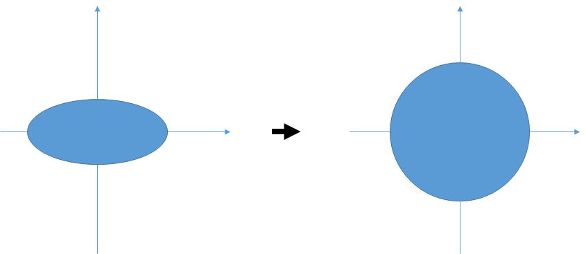
There are so many types of distance metric between two vectors or features. Euclidean Distance is the simplest.
$$\begin{equation} D_{Euclidean}(\mathbf{x})=\sqrt{(\mathbf{x}-\mathbf{y})^{T}(\mathbf{x}-\mathbf{y})} \end{equation}$$

As describe in the figure above, if we select euclidean distance, we don't care about the distribution of sample group and its covariances.

 
In the calculation of Mahalanobis Distance, normalization transform on bases is added just before Euclidean Distance calculation.
$$\begin{equation} D_{Mahalanobis}(\mathbf{x})=\sqrt[]{(\mathbf{x}-\mathbf{y})^{T}\mathbf{\Sigma}^{-1}(\mathbf{x}-\mathbf{y})} \end{equation}$$

Let's deep-dive into the $\Sigma^-1$.
We already look over covariance matrix $\Sigma$ in the previous article of PCA.

$$\begin{eqnarray*} \Sigma & = & \left[\begin{array}{ccc} \sigma_{11}^{2} & \cdots & \sigma_{1D}^{2}\\ \vdots & \ddots & \vdots\\ \sigma_{D1}^{2} & \cdots & \sigma_{DD}^{2} \end{array}\right]\\ & \Downarrow & diagonalization\\ & = & Q\varLambda Q^{T}\\ & = & \left[\begin{array}{cccc} \mathbf{e}_{1} & \mathbf{e}_{2} & \cdots & \mathbf{e}_{D}\end{array}\right]\left[\begin{array}{ccc} \lambda_{1} & \cdots & 0\\ \vdots & \ddots & \vdots\\ 0 & \cdots & \lambda_{D} \end{array}\right]\left[\begin{array}{c} \mathbf{e}_{1}^{T}\\ \mathbf{e}_{2}^{T}\\ \vdots\\ \mathbf{e}_{D}^{T} \end{array}\right] \end{eqnarray*}$$

$\lambda$s can be replaced with "NEW" variances, $\sigma^2$s.

$$\begin{eqnarray*} \Sigma & = & Q\varLambda Q^{T}\\ & = & \left[\begin{array}{cccc} \mathbf{e}_{1} & \mathbf{e}_{2} & \cdots & \mathbf{e}_{D}\end{array}\right]\left[\begin{array}{ccc} \sigma_{11}^{2} & \cdots & 0\\ \vdots & \ddots & \vdots\\ 0 & \cdots & \sigma{}_{DD}^{2} \end{array}\right]\left[\begin{array}{c} \mathbf{e}_{1}^{T}\\ \mathbf{e}_{2}^{T}\\ \vdots\\ \mathbf{e}_{D}^{T} \end{array}\right] \end{eqnarray*}$$
 
The matrix consisting of $\mathbf{e}^T_d$s means transformation to new bases ${\mathbf{e}_d}$.



$$\begin{eqnarray*} \Sigma^{-1} & = & Q\varLambda^{-1}Q^{T}\\ & = & \left[\begin{array}{cccc} \mathbf{e}_{1} & \mathbf{e}_{2} & \cdots & \mathbf{e}_{D}\end{array}\right]\left[\begin{array}{ccc} \frac{1}{\sigma{}_{11}^{2}} & \cdots & 0\\ \vdots & \ddots & \vdots\\ 0 & \cdots & \frac{1}{\sigma{}_{DD}^{2}} \end{array}\right]\left[\begin{array}{c} \mathbf{e}_{1}^{T}\\ \mathbf{e}_{2}^{T}\\ \vdots\\ \mathbf{e}_{D}^{T} \end{array}\right]\\ & = & \left(\left[\begin{array}{cccc} \mathbf{e}_{1} & \mathbf{e}_{2} & \cdots & \mathbf{e}_{D}\end{array}\right]\left[\begin{array}{ccc} \frac{1}{\sigma{}_{11}} & \cdots & 0\\ \vdots & \ddots & \vdots\\ 0 & \cdots & \frac{1}{\sigma{}_{DD}} \end{array}\right]\right)\left(\left[\begin{array}{ccc} \frac{1}{\sigma{}_{11}} & \cdots & 0\\ \vdots & \ddots & \vdots\\ 0 & \cdots & \frac{1}{\sigma{}_{DD}} \end{array}\right]\left[\begin{array}{c} \mathbf{e}_{1}^{T}\\ \mathbf{e}_{2}^{T}\\ \vdots\\ \mathbf{e}_{D}^{T} \end{array}\right]\right) \end{eqnarray*}$$

$\frac{1}{\sigma}$ means unit-varaince normalization.

Multivariate Normal Distribution

Multivariate Normal Distribution(MND) is :

$$\begin{equation} \mathcal{N}_{D}(\mu,\Sigma)=\frac{1}{\sqrt{2\pi^{D}\left|\Sigma\right|}}\exp\left(-\frac{1}{2}(\mathbf{x}-\mu)^{T}\mathbf{\Sigma}^{-1}(\mathbf{x}-\mu)\right) \end{equation}$$

where $D=\dim\left(\mathbf{x}\right)$.

We can see a term of squared Mahalanobis Distance. $(\mathbf{x}-\mu)^T\Sigma^{-1}(\mathbf{x}-\mu)$ means the squared Mahalanobis Distance from $\mu$. Determinant of $\Sigma$ is a product of variances $\prod_{d}\sigma_d^2$.

QDA (Quadratic Discriminant Analysis)

QDA is more general form of LDA. For QDA We need a important assumption that all classes have a normal distribution (MND).

If we want to discriminate class k and h, we have the following discriminant system.

$$\begin{equation} \frac{g_{k}(\mathbf{x})}{g_{h}(\mathbf{x})}>T_{k\text{ against }h} \end{equation}$$ $$\begin{eqnarray*} g_{k}(\mathbf{x}) & = & p(\mathbf{x}|C_{k})p(C_{k})\\ & = & \frac{1}{\sqrt{2\pi^{D}\left|\Sigma_{k}\right|}}\exp\left(-\frac{1}{2}(\mathbf{x}-\mu_{k})^{T}\mathbf{\Sigma}_{k}^{-1}(\mathbf{x}-\mu_{k})\right)p(C_{k}) \end{eqnarray*}$$ $$\begin{eqnarray*} \frac{g_{k}(\mathbf{x})}{g_{h}(\mathbf{x})} & = & \frac{\frac{1}{\sqrt{2\pi^{D}\left|\Sigma_{k}\right|}}\exp\left(-\frac{1}{2}(\mathbf{x}-\mu_{k})^{T}\mathbf{\Sigma}_{k}^{-1}(\mathbf{x}-\mu_{k})\right)p(C_{k})}{\frac{1}{\sqrt{2\pi^{D}\left|\Sigma_{h}\right|}}\exp\left(-\frac{1}{2}(\mathbf{x}-\mu_{h})^{T}\mathbf{\Sigma}_{h}^{-1}(\mathbf{x}-\mu_{h})\right)p(C_{h})}\\ & = & \frac{\left|\Sigma_{k}\right|^{-\frac{1}{2}}\exp\left(-\frac{1}{2}(\mathbf{x}-\mu_{k})^{T}\mathbf{\Sigma}_{k}^{-1}(\mathbf{x}-\mu_{k})\right)p(C_{k})}{\left|\Sigma_{h}\right|^{-\frac{1}{2}}\exp\left(-\frac{1}{2}(\mathbf{x}-\mu_{h})^{T}\mathbf{\Sigma}_{h}^{-1}(\mathbf{x}-\mu_{h})\right)p(C_{h})} \end{eqnarray*}$$

It is based on simple Bayesian Decision. Let's refine the formula by using log-scale and the general notation, $\pi_{k}=p(C_{k})$

$$\begin{eqnarray*} \ln\left(\frac{g_{k}(\mathbf{x})}{g_{h}(\mathbf{x})}\right) & = & -\frac{1}{2}\ln\left|\Sigma_{k}\right|+\left(-\frac{1}{2}(\mathbf{x}-\mu_{k})^{T}\mathbf{\Sigma}_{k}^{-1}(\mathbf{x}-\mu_{k})\right)+\ln\pi_{k}+\frac{1}{2}\ln\left|\Sigma_{h}\right|-\left(-\frac{1}{2}(\mathbf{x}-\mu_{h})^{T}\mathbf{\Sigma}_{h}^{-1}(\mathbf{x}-\mu_{h})\right)-\ln\pi_{h} \end{eqnarray*}$$

The discriminant function has a quadratic form of vectors. This shows why its name is "Q"DA.

LDA (Linear Discriminant Analysis)

LDA need one more assumption. $\Sigma$s are same.

It looks unrealistics. But here go ahead.

$$\begin{eqnarray*} \ln\left(\frac{g_{k}(\mathbf{x})}{g_{h}(\mathbf{x})}\right) & = & -\frac{1}{2}\ln\left|\Sigma\right|+\left(-\frac{1}{2}(\mathbf{x}-\mu_{k})^{T}\mathbf{\Sigma}^{-1}(\mathbf{x}-\mu_{k})\right)+\ln\pi_{k}+\frac{1}{2}\ln\left|\Sigma\right|-\left(-\frac{1}{2}(\mathbf{x}-\mu_{h})^{T}\mathbf{\Sigma}^{-1}(\mathbf{x}-\mu_{h})\right)-\ln\pi_{h}\\ & = & \left(-\frac{1}{2}(\mathbf{x}-\mu_{k})^{T}\mathbf{\Sigma}^{-1}(\mathbf{x}-\mu_{k})\right)+\ln\pi_{k}-\left(-\frac{1}{2}(\mathbf{x}-\mu_{h})^{T}\mathbf{\Sigma}^{-1}(\mathbf{x}-\mu_{h})\right)-\ln\pi_{h}\\ & = & -\frac{1}{2}\left(\mathbf{x}^{T}\mathbf{\Sigma}^{-1}\mathbf{x}-2\mu_{k}^{T}\mathbf{\Sigma}^{-1}\mathbf{x}+\mu_{k}^{T}\mathbf{\Sigma}^{-1}\mu_{k}\right)+\frac{1}{2}\left(\mathbf{x}^{T}\mathbf{\Sigma}^{-1}\mathbf{x}-2\mu_{h}^{T}\mathbf{\Sigma}^{-1}\mathbf{x}+\mu_{h}^{T}\mathbf{\Sigma}^{-1}\mu_{h}\right)+\ln\pi_{k}-\ln\pi_{h}\\ & = & -\frac{1}{2}\left(-2\mu_{k}^{T}\mathbf{\Sigma}^{-1}\mathbf{x}+\mu_{k}^{T}\mathbf{\Sigma}^{-1}\mu_{k}\right)+\frac{1}{2}\left(-2\mu_{h}^{T}\mathbf{\Sigma}^{-1}\mathbf{x}+\mu_{h}^{T}\mathbf{\Sigma}^{-1}\mu_{h}\right)+\ln\pi_{k}-\ln\pi_{h}\\ & = & (\mu_{k}-\mu_{h})^{T}\mathbf{\Sigma}^{-1}\mathbf{x}-\frac{1}{2}(\mu_{k}+\mu_{h})^{T}\mathbf{\Sigma}^{-1}(\mu_{h}-\mu_{k})+\ln\pi_{k}-\ln\pi_{h} \end{eqnarray*}$$

As you see, the discriminant boundary changes from a curve to a straight line (Linear)

Conclusion

Covariance matrix is everywhere. The contents described here are so feasible that most of researchers and developers do not need to check again. But someone who doesn't have concrete mathematical or statistical funcdamentals cannot catch these common pieces and can be confused easily.